What is MultiCollinearity and how to resolve it?

3 min readApr 26, 2021

https://kaiserm.medium.com/how-to-tackle-multicollinearity-79afe58e9479

Q1: What is MultiCollinearity?

If any of our Independent Feature(x1,x2) is internally co-related more than 90%.

Q2: How multicollinearity works and how to resolve it?

lets say we are solving Regression/classification problem where we have 10–15 features. i.e (n rows, 15 features) n x 15.

Step 1: we plot correlation heat map by comparing each feature with each other.

Step 2: So,lets say after doing step 1 we got features[f3,f4] which are highly correlated with more than 90%.

Step 3: So, what we can do is remove any one of the feature which has [p-value > 0.05]

Important Note: It is not Possible for finding correlation for each feature if we have large amount of features such as , eg: (n rows,200 features) n x 200. So to solve that issue we use something called Ridge and Lasso Regression.

Lets take example:

df = pd.read_csv(“Advertising.csv”)
X = df[[‘TV’, ‘radio’, ’newspaper’]] #Independent Features
y = df[‘sales’] #Dependent Features
df.head()

y = b0 + b1x1 + b2x2 + b3x3

x1 = TV , x2 = radio , x3 = newspaper , y = sales
        b0 = Intercept
        b1,b2,b3 = Slopes or Coefficient

So in order to check if there is Multi Collinearity issue or not we will use OLS MODEL : Ordinary Least square.

import statsmodels.api as sm
X = sm.add_constant(X) # add B0 with all const values
X.head()

model= sm.OLS(y, X).fit()
model.summary()

import matplotlib.pyplot as plt
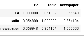
X.iloc[:,1:].corr()

Conclusion: None of Features are internally corelated, all features(Tv, Radio,Newspaper) having values nearer to zero,i.e. all independent features are not correlated to each other.

2:

df1 = pd.read_csv(‘Salary_Data.csv’)
df1.head()

X = df1[[“YearsExperience”,”Age”]]
y = df1[‘Salary’]

Using OLS model